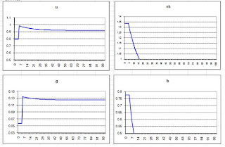
In the case of perfect foresight, the steady state of the SIMEX model and the SIM model are identical. The national income in both steady states will be the same.
In the case, however, where mistakes are made in expectations, a steady state will be reached at a slower rate of convergence than the perfect foresight case. This slower rate is due to the recursive nature of the SIMEX model and the extra time needed to ease the discrepancy between desired and realized holdings of money. The path to reach this state will be different. The disposable income reached will be identical. Actual wealth however, in the steady state where expectations have been made incorrectly, will be higher.
Relating this to the real world, if a household underestimates its income, there will be an increase in savings and therefore an increase in the stock of wealth (H). This change in wealth will cause consumption to increase at a rate higher than if the income expectation had been correct. The household’s consumption in a certain period won’t increase as they have prepared to consume a certain amount so they will find themselves with an unexpectedly excessive or depleted and therefore amend their consumption decisions. In an economy where the disposable income of the household is continually underestimated, public debt would, as a result, be larger than that of an economy where perfect expectations are made.

As shown in Table above. We start from a situation where there is no economic activity whatsoever, and where none has ever existed, in period 1. Households have no income, and they never accumulated any wealth. In period 2, households assume an income level of 30, and hence expected disposable income is equal to 24(=30-(0.2*30)). Since there is a marginal propensity to consume of 0.6, the actual consumption is 14.4(=α1*YDe=0.6*24) and hence income is 44.4(=G+C=30+14.4). The discrepancy between desired and realized holdings of money is equal to the discrepancy between expected and realized disposable income. Also, one can see that the expected disposable income at period 3 is the same as realized disposable income at period 2.
Question 2
(i) The consumption function in the standard ISLM model includes an autonomous component. Consumption is equal to autonomous consumption (consumption that will happen anyway) plus the product of the marginal propensity to consume and disposable income. Current consumption is not related to previous stocks of wealth.  The specification of the consumption function in SIM is different and consumption is a function of stocks and flows. Consumption is calculated as some proportion alpha one of the flow of disposable income plus a smaller proportion alpha two of the stock of wealth from the previous period.
  A version of SIM that replicates the ISLM could be created by allowing consumption to be a function of autonomous consumption (which is independent of current income), the marginal propensity to consume and disposable income only as the ISLM model does not consider stocks such as the stock of money.
(ii)The equilibrium value of Y* calculated using a standard multiplier such as that in the ISLM represents a short run equilibrium. It does not represent a steady state solution.
However the form of SIM that replicates the ISLM model uses the specification of the consumption function mentioned above and it can reach a stationary state. It is possible for the average propensity to consume to be unity and this means that we can have consumption equal to disposable income in the stationary state. This can occur even if the marginal propensity to consume is less than one. In this case autonomous spending has a similar role to that of consumption from the stock of previous wealth and ensures the stability of the model. If the autonomous part was ignored the model would be unstable as the stock of money and government debt would rise forever.


 After
After
After


1 comment:
Excellent summary, especially with the ZFS model.
Post a Comment